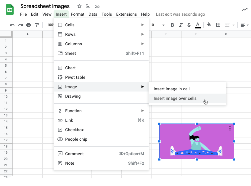
In the realm of Google Sheets, incorporating images into cells is a common task. The conventional approach involves navigating to the “Insert” option, selecting “Image,” and specifying either the image file or its URL.
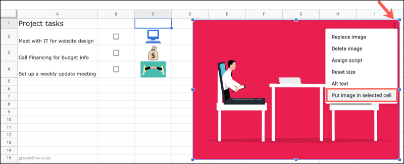
However, this technique treats the image as a detached object, preventing it from adjusting or resizing along with the cells. If the cell containing the image is deleted, the image remains unaffected. Similarly, resizing cells won’t impact the image’s dimensions (as demonstrated below):
Dealing with this can be quite bothersome, especially when working with numerous images in Google Sheets.
A Better Way to Insert Images in Google Sheets Cells
Thankfully, Google Sheets offers some nifty functions, such as the “IMAGE” function, which can directly insert an image into a cell using its URL.
Yes, it’s that straightforward!
First, let’s delve into the details of the “IMAGE” function.
Syntax:
IMAGE(url, [mode], [height], [width])
– “url” stands for the URL of the desired image to be inserted into the cell.
– “[mode]” is an optional argument that determines how the image fits within the cell. Four options are available:
– Mode 1: Resizes the image to fit inside the cell while maintaining the aspect ratio. If left empty, 1 is the default.
– Mode 2: Stretches or compresses the image to fit the cell, disregarding the aspect ratio.
– Mode 3: Leaves the image at its original size, which may lead to cropping.
– Mode 4: Allows custom size specification.
– “[height]” (applicable for Mode 4) enables you to specify the image’s height in pixels.
– “[width]” (applicable for Mode 4) enables you to specify the image’s width in pixels.
Now, let’s observe a real-world example.
For demonstration purposes, we’ll use the Amazon logo, whose URL is as follows:
https://images-na.ssl-images-amazon.com/images/G/01/SellerCentral/legal/amazon-logo_transparent.png
In the desired cell, enter the following formula:
=IMAGE(“https://images-na.ssl-images-amazon.com/images/G/01/SellerCentral/legal/amazon-logo_transparent.png”)
Ensure the URL is within double quotes.
The outcome will be as follows:
Since we didn’t specify a mode argument, the image automatically resized to fit the cell.
Now, let’s explore how different mode arguments affect the same image:
– Mode 1: The image resizes to fit the cell.
– Mode 2: The image stretches to fit the cell, ignoring aspect ratio.
– Mode 3: The image appears at its original size, causing the top to be cropped.
– Mode 4: The image adopts user-defined height and width (in pixels). Note that without height and width arguments, Mode 4 will trigger an error.
Benefits of Using the IMAGE Function
While you can also insert images using the “Insert Image” option in Google Sheets (located in the “Insert” tab), the “IMAGE” function offers several advantages:
1. The “IMAGE” function keeps the image within the cell, even when rows or columns are resized. It also hides the image if the cells are hidden. In contrast, the “Insert Image” feature places the image as a floating object on the worksheet, without automatic resizing or hiding.
2. The “IMAGE” function allows dynamic usage by incorporating cell references. If the URL in the cell changes, the “IMAGE” function automatically updates to display the image of the updated URL.
Creating a Dynamic Image Lookup in Google Sheets
Let’s explore an example where the “IMAGE” function in Google Sheets can perform an Image Lookup.
Imagine you’re developing an interactive dashboard where users can choose a company name, and the dashboard updates with the selected company’s details.
You can employ the “IMAGE” function for an image lookup, ensuring that the logo automatically updates when a company is selected, as shown below:
Here’s how to create it in Google Sheets:
1. Compile a list of company names along with their respective image links.
2. In your interactive dashboard or report, create a dropdown menu using the company names (e.g., in cell A1).
3. In cell B1 (where you want the image lookup functionality), utilize the following “VLOOKUP” formula: =IMAGE(VLOOKUP(A1,Sheet2!$A$2:$B$6,2,FALSE),1).
And that’s it!
Now, when you change the company name in cell A1, the image will automatically update accordingly.
I hope you found this tutorial helpful. Please feel free to share your thoughts in the comments section below.