Did you know that the checkbox originated in the Roman Empire, derived from the word Veritas, which means truth, to V? It later evolved to resemble the tick we know today.
Checkboxes are a fantastic method for keeping track of data, and Google Sheets now offers a simple way to insert checkboxes into cells.
In this tutorial, I’ll cover everything you need to know about using Google Sheets checkboxes, along with some helpful examples.
Adding a Checkbox in Google Sheets
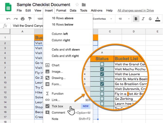
Follow these steps to insert a checkbox in Google Sheets:
1. Choose the cell where you want to add the checkbox.
2. Click on the “Insert” option in the menu.
3. Select “Checkbox” from the options.
By following these steps, you will successfully insert a checkbox in the selected cell. If you want to add checkboxes to multiple cells, simply select the cells and insert the checkbox.
It’s worth noting that checkboxes in Google Sheets function like text in a cell, allowing you to customize their size, color, and font. Additionally, you can modify cell values in the data validation window.
Using the Google Sheets Checkbox
Once you’ve inserted a checkbox in Google Sheets, you can use it by merely clicking on it.
The checkbox functions as a toggle. When you click once, it gets checked, and clicking again will uncheck it.
While the checkbox appears in the cell, the backend process involves cell value changes:
– When checked, the cell value becomes TRUE.
– When unchecked, the cell value becomes FALSE.
These value changes enable various functionalities with checkboxes in Google Sheets, such as:
– Creating a to-do list and marking tasks as done/complete.
– Highlighting specific data points based on selection (e.g., top/bottom 10).
– Creating interactive charts in Google Sheets.
You can download one of our Google Sheets checkbox templates below.
[Checkbox template link]
Now, let’s delve into the examples in detail.
Example 1 – Creating a To-Do List with Conditional Formatting
The following example demonstrates how to insert checkboxes in Column B, which, when checked, changes the corresponding item’s color in Column A and applies the strikethrough format.
This can be achieved using conditional formatting. The key is using the TRUE/FALSE values in the checkbox cells to trigger the formatting.
Follow these steps to create this:
1. Select the cells in Column A (containing the items) or use the keyboard shortcut CTRL + Enter for an entire column.
2. Click the “Format” button in the menu.
3. Choose “Conditional Formatting” from the options.
4. In the Conditional Formatting pane, click the “Format cells if” drop-down.
5. Select “Custom formula is.”
6. Enter the following formula: =$B2
7. Specify the format (color and strikethrough).
The above technique applies conditional formatting whenever the formula returns TRUE, which happens when the checkbox is checked.
Example 2 – Highlighting Data Using Checkboxes and Conditional Formatting
Suppose you have a dataset of students’ marks. You can add a checkbox to highlight students who scored more than 85 in green and/or students who scored less than 35.
Follow these steps to achieve this:
1. Select the cells in Column B (containing the marks).
2. Click the “Format” button in the menu.
3. Choose “Conditional Formatting” from the options.
4. In the Conditional Formatting pane, click the “Format cells if” drop-down.
5. Select “Custom formula is.”
6. Enter the following formula: =AND($E$3,B2>=85)
7. Specify the format for marks above 85 (use green color in the example).
8. Click “Done.”
9. Click “Add New Rule.”
10. In the Conditional Formatting pane, click the “Format cells if” drop-down.
11. Select “Custom formula is.”
12. Enter the following formula: =AND($E$4,B2<35)
13. Specify the format for marks below 35 (use red color in the example).
14. Click “Done.”
The above steps use formulas to check two conditions:
1. Whether the cell value is greater than or equal to 85 or less than 35.
2. Whether the checkbox is checked or not.
When both conditions are met, the cell gets highlighted.
Example 3 – Creating an Interactive Chart with Checkboxes
Let’s say you have profit margin data for a company, and you want to plot the data for 2018. Additionally, you want to give users the option to plot the data for 2017 or 2019 using checkboxes.
To do this, you need a dataset that depends on the checkboxes. For instance, if the 2017 checkbox is checked, the corresponding data should be available; otherwise, it should be blank.
Follow these steps to create this interactive chart:
1. Create a new dataset as shown below, with the order changed to (2018, 2017, and 2019F).
[New dataset image]
2. Now, for each year, use the following formulas:
For 2018:
=B3 (returns 2018 values)
For 2017:
=IF($H$4,B2,””) (H4 contains the checkbox for 2017; the formula returns the value from the original dataset if the checkbox is checked, else it returns a blank)
For 2019F:
=IF($I$4,B4,””) (I4 contains the checkbox for 2019; the formula returns the value from the original dataset if the checkbox is checked, else it returns a blank)
3. Insert checkboxes in cell H4 and I4.
4. Create a combo chart using the data created with the formulas:
– Select the data.
– Click the “Insert” option in the menu.
– Click on “Chart.”
– In the Chart editor pane, change the Chart type to “Combo.”
Now, the chart will automatically update when you check/uncheck the checkboxes.
How to Check and Uncheck All Boxes In Google Sheets
After creating the checkboxes, you can easily check and uncheck them all with the following steps:
1. Highlight the column with the checkboxes by clicking on the column header (for the entire spreadsheet, use the Ctrl + A keyboard shortcut).
2. Press Enter to toggle the checkboxes on or off.
How to Add Checkboxes in Google Sheets With the Fill Handle
You can quickly create checkboxes in Google Sheets by clicking and dragging the small blue box after selecting a cell with a checkbox. This copies the checkbox into adjacent cells.
Using Data Validation to Add Custom Values to Checkboxes in Google Sheets
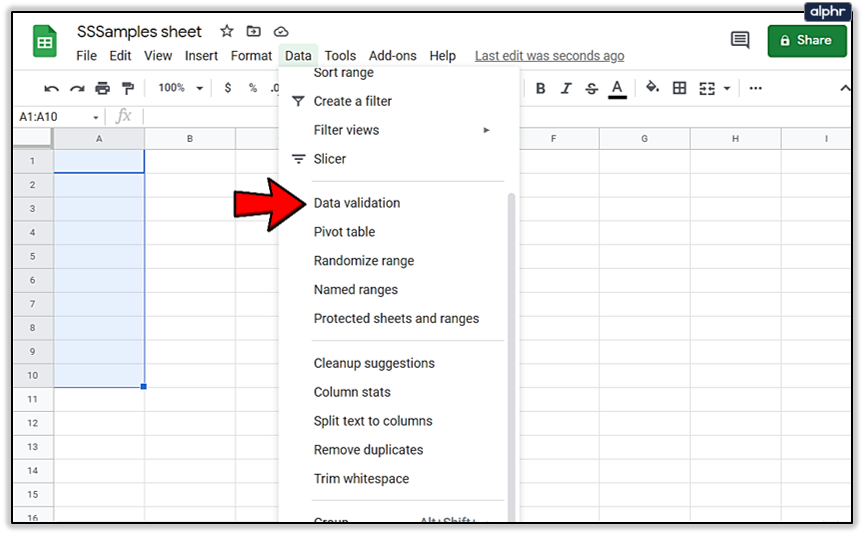
If you prefer to use the Data menu instead of inserting checkboxes, you can add custom values to them using data validation:
1. Navigate to Data > Data validation.
2. In the menu that appears, change the Criteria to Checkbox.
3. Check the “Use custom cell values” option.
4. Define what the checked and unchecked boxes represent in your sheet.
How to Remove Custom Values From a Checkbox
To remove custom values, go back to the data validation menu and uncheck “use custom cell values.”
Example 4: How To Add Google Sheets Checkbox with App Scripts
Using App Scripts is an excellent way to create automated choices for your checkboxes. Here’s how you can do it:
1. Access App Scripts in Extensions on the toolbar.
2. Input the checkbox function in the script. You can copy-paste the following code:
[App Script