Pivot tables have long been a valuable tool for those diving into vast quantities of data, offering a unique approach to group, sort, and analyze data points. If you’re familiar with them, you’re aware of their capabilities in collating large datasets.
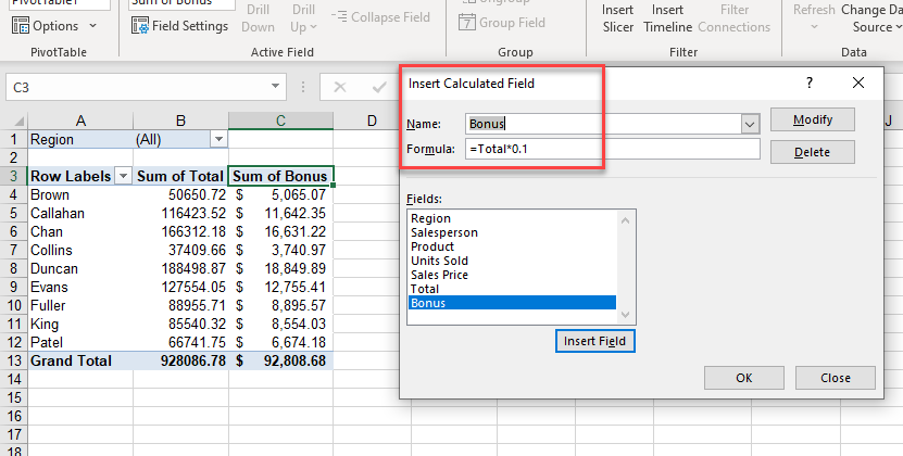
A standout feature? The inclusion of the ‘Calculated Field’ function, enabling you to infuse personalized formulas and functions, elevating the depth of your analysis.
In this guide, we’ll delve into the ins and outs of utilizing calculated fields within pivot tables, unveiling their true potential.
Understanding Calculated Fields in Google Sheets
Typically, a pivot table is replete with built-in metrics like average, sum, median, and variance, which are foundational for data analysis. But sometimes, these may not cater to specific calculations you have in mind.
Enter Calculated Fields. These fields augment your pivot tables by allowing you to design unique computations not found in the standard options. Think of wanting to integrate a VAT to the sales figures of a branch’s items. While this could be integrated into the main dataset, calculated fields allow this addition exclusively within the pivot table, ensuring the original data remains pristine.

Steps to Harness Calculated Fields in Google Sheets Pivot Tables
Imagine having a dataset and wanting to:
1. Showcase total sales of various products.
2. Display the total sales augmented by a 5% value.
3. Highlight the minimum units sold per item.
To actualize this:
1. Generating a Pivot Table for Total Product Sales:
– Click on ‘Data’ in the menu.
– Select ‘Pivot Table’ from the ensuing dropdown.
– Opt for either a new sheet or the existing one for the pivot table. For clarity, a new sheet is suggested.
– Initiate by clicking ‘Create’.
– You’ll now see a grid with ‘Rows’, ‘Columns’, and ‘Values’.
– With the Pivot Table Editor’s assistance, populate the table: ‘Item’ for rows and ‘SalesPrice’ for values, showing each product’s total sales.
2. Incorporating a 5% VAT using a Calculated Field:
– Click anywhere within your pivot table.
– Under ‘Values’, click ‘Add’ and pick the ‘Calculated field’.
– Rename this field to ‘Total with VAT’.
– Within the Pivot table editor, insert the formula: =SalesPrice + (5/100 * SalesPrice) to reflect the 5% increase.
3. Depicting Minimum Units Sold via another Calculated Field:
– Repeat the initial steps as above to add another calculated field.
– Rename this to ‘Smallest Units Sold’.
– For the formula, use: =MIN(Units).
– Modify ‘Summarize by’ to ‘Custom’ to see the results.
Key Takeaways on Calculated Fields
As enriching as calculated fields are, they come with specifics:
– Formulas should reference the original dataset cells and not totals or subtotals of the pivot table.
– Field names from the dataset should be used. Avoid cell addresses or individual cell names.
– Field names in formulas should be accurate. If it’s a multi-word name with spaces, encapsulate it with single quotes.
Conclusively, this guide has unraveled how pivot tables, coupled with calculated fields, can be a powerhouse for data analysis. These fields bolster the dynamism of pivot tables, allowing for tailored summaries. Here’s to your enhanced data exploration journey!