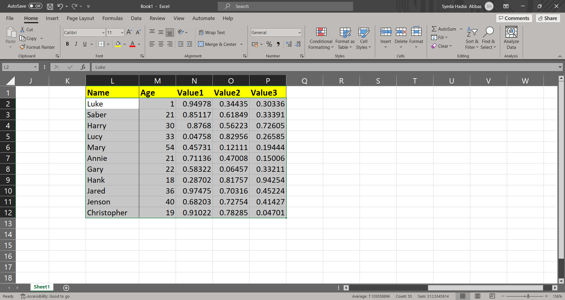
While the dominance of Microsoft Excel remains unchallenged in the realm of spreadsheets, Google Sheets has been gradually gaining ground. It has garnered a following among freelancers, small business proprietors, and entrepreneurs. Though it may not yet possess the data-crunching prowess of Excel or the task-automation capabilities of VBA, it boasts distinct advantages over Excel spreadsheets.
Google Sheets vs. Excel: A Comparison
Google Sheets, being web-based, offers easy accessibility across devices and locations. Seamlessly, you can transition from desktop/laptop work to smartphone edits using the Google Sheets app, thanks to its cloud-based setup.
Collaboration is a standout feature, allowing multiple individuals to collaborate on a Google Sheets document simultaneously, eliminating the hassles of constant emails and version control concerns.
An intriguing feature involves real-time chat among users accessing a Google Sheets document.
However, while Google Sheets presents a cost-effective option for basic data entry and management tasks (freelancers, small businesses, educators, etc.), it falls short of Excel in intricate data analysis, charting, and automation capabilities.
Moreover, Google Sheets harbors an array of practical functions and functionalities that bolster its utility.
Anticipating a Shift in the Spreadsheet Landscape
Google Sheets’ trajectory suggests it’s poised to become a significant player in the spreadsheet arena, transcending its current standing.
Discovering Google Sheets Hacks
For those embracing Google Sheets, here’s a collection of 10 tips and tricks designed to streamline your workflow and heighten productivity.
1. Effortlessly Enhance Readability with Alternating Row Colors

Did you know that introducing alternating row colors in a dataset dramatically improves its legibility? Google Sheets offers a built-in feature called conditional formatting that achieves this effect.
To rapidly implement alternating row colors in Google Sheets:
– Highlight the target dataset.
– Navigate to the Format tab and select ‘Alternating Colors.’
– Tailor the formatting style and establish the presence of headers/footers. Custom formats can also be created.
This method instantaneously applies the chosen colors to alternate rows in your Google Sheets. To undo this effect, utilize the ‘Remove Alternating Colors’ option.
2. Seamlessly Lock Rows/Columns with a Simple Drag-and-Drop Technique
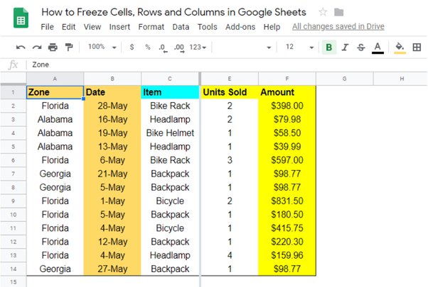
Tackling extensive datasets often leads to navigation challenges, especially when headers disappear upon scrolling. Freezing rows or columns ensures these headers remain visible, enhancing data orientation.
For instance, to freeze the top row in Google Sheets:
– Locate the gray empty box in the top-left corner.
– Position the mouse on the thick gray line beneath the box, triggering the hand icon.
– Left-click and drag the line downwards to freeze the top row.
Akin to this, freezing other rows or columns is equally straightforward. Google Sheets simplifies this process compared to Excel’s ribbon-based freezing.
3. Instantly Embed Images via URLs

Google Sheets introduces a unique function that directly embeds images using their URLs, a capability absent in Excel—at least as of my last update.
Leverage the IMAGE function with the following syntax:
=IMAGE(URL, [mode], [height], [width])
Arguments include:
– URL: The image’s URL.
– [mode]: Optional value (1 to 4) dictating image display (resize, stretch, original size, or customized dimensions).
– [height]: Image height.
– [width]: Image width.
For example, inserting the Google logo:
=IMAGE(“https://www.google.com/images/srpr/logo3w.png”)
4. Elevate Data Entry with Dropdown Lists
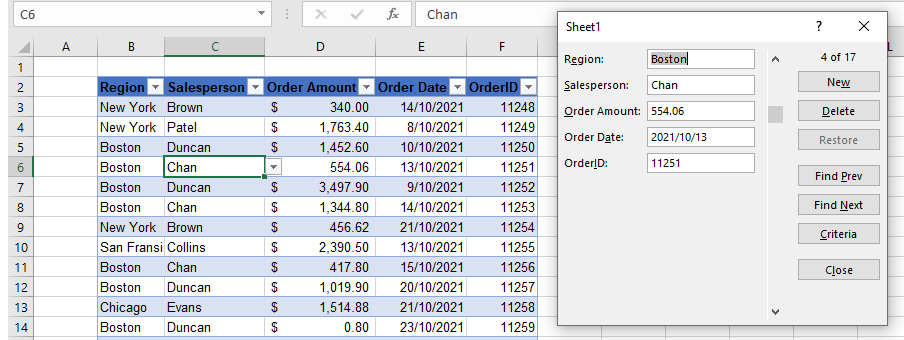
Dropdown lists enhance user-friendly data entry, ensuring pre-defined items are selected. This consistency minimizes errors and inconsistencies, often encountered in manual entry.
Implementing a dropdown list in Google Sheets:
– Choose the target cell.
– Access the Data tab and select Validation.
– Customize the criteria, referring to the cell range and pre-defined options.
This generates a dynamic dropdown, which adapts as source data changes. An arrow indicates the dropdown’s presence, simplifying selection.
5. Swiftly Extract Distinct Items
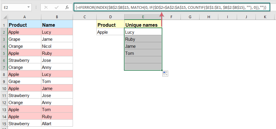
Handling datasets with duplicates becomes smoother using Google Sheets’ UNIQUE function. If you seek unique elements within a dataset, the UNIQUE function is invaluable.
For instance, to extract unique names from a list:
=UNIQUE(A1:A10)
6. Eradicate Spelling Mistakes with Spell Check
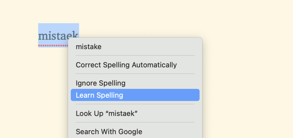
Accurate language usage in your work is pivotal. Google Sheets simplifies this through its built-in spell-check feature, ensuring you’re free of typographical errors.
Employ the following steps for spell-check:
– Select the relevant data or the entire sheet.
– Access the Tools tab and click on Spelling.
Rectify or ignore the suggested corrections as needed.
7. Seamlessly Merge Sheets from Different Documents
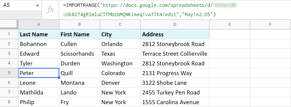
Combining multiple trackers or to-do lists into one master sheet proves convenient. Google Sheets facilitates this by allowing you to copy sheets across documents.
To achieve this:
– Open the source document.
– Right-click the sheet to copy.
– Choose ‘Copy to…’ and select the target document.
The copied sheet now resides in the destination document.
8. Zooming Insights

Zoom functionality enhances data visibility and analysis. While Google Sheets lacks a dedicated zoom for its work area, it accommodates zooming the entire browser window.
To zoom in Google Sheets (Chrome browser):
– Click the ‘Chrome customize’ icon in the top-right.
– Adjust the zoom level using +/- buttons.
9. Integrate Hyperlinks with Ease
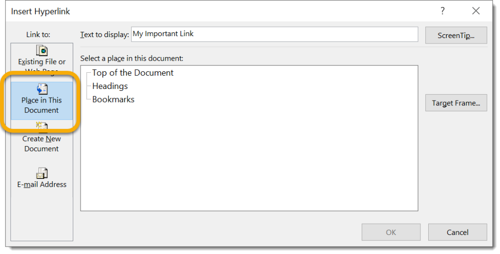
The HYPERLINK function streamlines hyperlink integration in Google Sheets. Ideal for connecting URLs to specific text, it avoids manual insertion.
The formula syntax is:
=HYPERLINK(URL, LINK_LABEL)
Where:
– URL: Full URL enclosed in quotes.
– LINK_LABEL: Text display for the hyperlink, enclosed in quotes.
Example:
=HYPERLINK(“https://www.google.com”,”Google”)
Hover over the hyperlink-enabled cell to access the link. Clicking the link transports you to the designated URL.
10. Swiftly Transpose Data
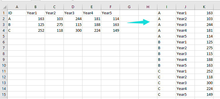
Like Excel, Google Sheets supports transposing data through Paste Special options. Transposition converts rows into columns and vice versa.
To transpose data in Google Sheets:
– Highlight and copy the desired data.
– Select the cell for transposed data.
– Right-click and access Paste Special, then choose Paste Transpose.
Note that formatting isn’t carried over, and you may need to manually copy formatting. Additionally, transposed data remains static; changes in source data necessitate repeating the process.
Embrace the Path to Enhanced Efficiency
These 10 Google Sheets techniques augment daily productivity, illustrating the software’s potential. Share your own tips and tricks in the comments—your insights could enrich others’ experiences.
