In this guide, we delve into the steps for freezing a row in Google Sheets. Through an easy-to-follow process complete with screenshots, you can secure the top row in your worksheet. This is particularly useful when working with large data chunks requiring lots of scrolling. The guide also covers freezing columns, noting that locking rows at the top or particular columns allows them to stay visible at all times.
Are you prepared to learn about freezing a row in Google Sheets? Let’s dive in.
Watch Video – How to Freeze a Row on Google Sheets (Lock a Row in Google Sheets)
The Essence of Freezing a Row in Google Sheets
What does it mean to freeze a row in Google Sheets? Quite simple, freezing entails securing cells at a particular location. As such, when you scroll through your worksheet, the frozen cells stay in one place. Regular spreadsheet users often freeze cells when handling large data quantities, allowing the cells or panes to remain visible when scrolling.
This function is beneficial when comparing data or maintaining track of information without the need to scroll back and forth. It also enhances the aesthetic appeal of your spreadsheets, such as concealing columns or rows.
Additionally, freezing rows lets you establish a header row or page titles on Google Sheets. Consequently, every printed page will feature the frozen row as the header. We’ll demonstrate two ways to ensure the top row of Google Sheets is constantly visible.
Method of Freezing a Row on Google Sheets
Google Sheets can ensure the top row stays visible:
In the above instance, the top row in Google Sheets remains visible as the initial row is frozen. While navigating through the data set, you can still see what you’re working on. This tutorial will illustrate two ways to pin rows in Google Sheets. Note that this is distinct from pinning a location in Google Maps, a topic we’ve recently discussed.
Using the Mouse to Freeze the Top Row in Google Sheets
Google spreadsheets can swiftly freeze rows using this method. It is also applicable when you want Google Sheets to freeze several rows.
You’ll need to move to the sheet’s top left section where an empty gray box is located. Observe the two thick gray lines in the box (on the right and left sides).
Hover your mouse over the gray line, and when the hand icon appears, left-click and drag it downwards.
The above action will immediately freeze a row in Google Sheets above the gray line, creating sticky Google Sheets row(s), as illustrated below:
This method can’t be used in Google Sheets to freeze a row in the center. It only allows freezing from the top downwards.
How to Freeze Columns in Google Sheets
Both previously mentioned methods can also be used to freeze columns in Google Sheets. You just have to adjust the horizontal gray line instead of the vertical one or choose the column options from the view options menu, which we’ll discuss in the next method.
Locking a Row in Google Sheets Using View Options
While the mouse method (detailed above) is incredibly convenient, there is an alternative way to freeze rows in Google Sheets.
Here’s how:
Select the cell in the column where you want the rows to be frozen up to. For instance, if you want the top five rows frozen, select the cell in row 5.
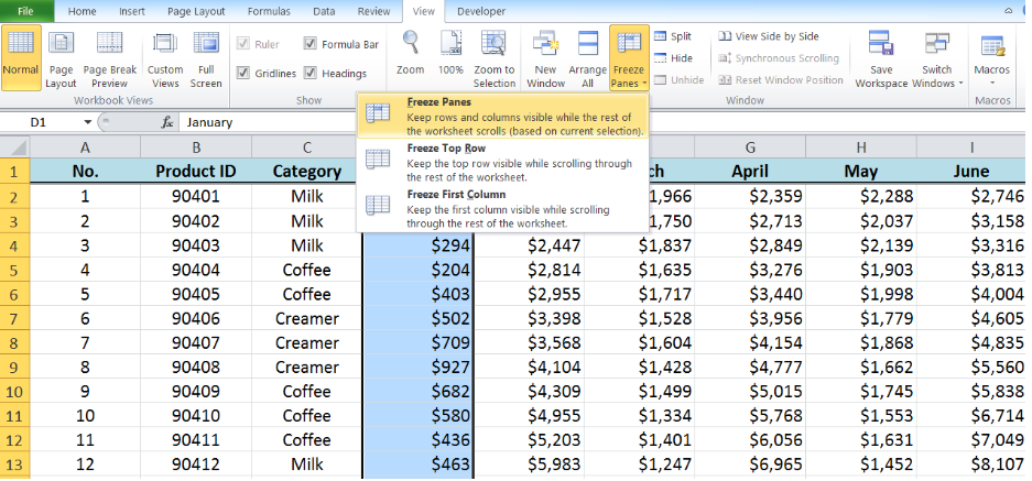
Navigate to View –> Freeze –> Up to Current Row (5). Note that the number in the parenthesis changes based on the selected cell.
This will freeze all the rows including and above the one chosen. This is handy if you want to freeze more than two rows. If you’re unsure about freezing the top row in Google Sheets, there are 2 standard options. You can either freeze the top row or the top two rows.
By repeating the above process, you can freeze a column in a Google spreadsheet. In the view menu, you have similar options for rows and columns. If you want to freeze one column, simply select 1 column in the view menu.
The frozen column should stay visible when you scroll down. If you want to freeze several columns, use the ‘up to current column’ option. This is an alternative way to freeze a column in Google Sheets. If you want to unfreeze columns, return to the view menu and select ‘no columns’ under the freeze option.
Freezing Multiple Rows
Both of the above methods work for freezing more than one row. Just make sure the gray line is over all the rows you want to have frozen. The same applies to columns.
Freezing Panes in Google Sheets
A pane is a combination of rows and columns in Google Sheets. If you’d like to learn how to freeze rows and columns in Google Sheets, all you have to do is both freeze the rows and freeze the columns with either of the methods we discuss in this article.
Freezing and Unfreezing Rows and Columns on Mobile
You can also freeze rows in sheets on your mobile phone, whether on Android or IOS. This will require you to download the Google Sheets app on your respective app store if you don’t already have it.
Android
Press and hold the row or column you want to freeze
Tap Freeze or unfreeze on the menu that pops up
iOS
- Tap the row number or the column letter
- Tap the right arrow that appears
- Tap freeze or unfreeze
- Unfreezing Rows in Google Sheets
Again, there are two ways to unfreeze after you freeze a row in Google Sheets:
Using a Mouse: Hover the mouse over the thick gray line that appears right below the last row that has been frozen. Left-click and drag it to bring it to the top. This will unfreeze all the frozen rows.
Using View Options: Go to View –> Freeze –> No Rows.
Frequently Asked Questions
Can You Freeze a Single Cell in Google Sheets?
Yes, here’s how to freeze cells in Google Sheets. You simply have to freeze the row and the columns. But this will only allow you to freeze cell A1. You can’t freeze a random cell.
How Do I Freeze a Specific Row in Google Sheets?
You can freeze a specific row in Google Sheets by selecting the row and going to “filter views” then freeze then choosing 1 row in the menu. Your frozen row should remain on the screen when you scroll down.
Can You Freeze Panes on Google Sheets?
Yes, you can freeze panes on Google Sheets to lock rows and columns. To learn more, you can read our article above. Otherwise, check Google’s advice on how to freeze or merge rows.
Conclusion
Freezing rows in Google Sheets is a simple solution to several problems. There are two paths to freezing a row in Google Sheets: using the mouse and using the view option. This is just one of the many other tips and tricks for Google Sheets we have for you. We hope this tutorial was helpful for you, and that you are now an expert on how to freeze rows in Google Sheets, as well as how to freeze columns. You might also be interested in how to delete every other row in Google Sheets.