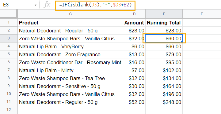
Ever wanted to grasp the sum progression in a series of numbers? Running totals give you a snapshot of such a sequence, presenting the ongoing sum at each step.
These totals aren’t just academic; they’re instrumental in realms of business and education.
Let’s delve into creating a running total in Google Sheets. You’ll employ the trusty SUM Function to do so.
Table of Contents
ToggleWhat Exactly is a Running Total?
Picture a running total as an evolving sum, tallying numbers sequentially. Each time a new digit joins the party, the total inflates by that amount. This mechanism not only provides insights into the growth trajectory but also lets you spot the aggregate by peeking at the final value.
From tracking company revenue, expenditure, stock counts, to logging employee hours, the utility of running totals in the corporate sphere is undeniable.

Achieving Running Totals in Google Sheets
To paint a clearer picture, let’s use a hypothetical dataset:
Our spotlight will be on column B (tagged as “Daily Expenditure”) where we’ll be introducing our running totals.

Harnessing the SUM Function for Running Totals
Our strategy involves using the SUM function. Let’s say you wish to discern the running total up to row 9. The formula would look something like:
=SUM($B$2:B9)
This will aggregate values from the second row to the ninth. Notice the use of dollar signs ($) with the starting cell? It stays fixed, whereas the ending cell remains flexible.
Why? This approach ensures the sum kicks off from a fixed point while allowing it to expand with every row.
Follow these instructions to nail the **Running Total for Daily Expenditure** in the third column:
1. In cell C2, punch in the formula: =SUM($B$2:B2).
2. Spot the fill handle at the bottom-right of cell C2? Drag it. This action replicates the formula throughout column C.
3. Voila! Column C now mirrors the running totals of column B.
Distinguishing Between Absolute & Relative Cell References
While the term may sound a tad technical, it’s quite simple. References in cells can either change with movement (relative) or stay anchored (absolute). The dollar sign ($) demarcates an absolute reference, e.g., $B$2.
For clarity, imagine two cell references pointing to the value in cell A1:
A1 (This one’s relative)
$A$1 (Absolutely unwavering)
While they seem identical, dragging them reveals their true nature. The relative one adjusts, but the absolute stays loyal to its initial reference.
Decoding the Formula
In C2, we have =SUM($B$2:B2). It’s calculating from B2 to B2. So, you get 72.34.
Move to C3, it morphs into =SUM($B$2:B3). Now, it totals the first couple of entries under Daily Expenditure. With every row, the range of this sum expands, finally presenting the aggregate of the whole Daily Expenditure list.
Automating Your Running Total
If copying the formula for each new entry feels tedious, throw in an IF statement. Ensure the running total pops up only when there’s an entry in the Daily Expenditure.
In C2, modify the formula:
=IF(B2<>””,SUM($B$2:B2),””)
Clone this formula down column C. When column B gets a new number, column C instantly updates the running total.
This guide equipped you with the skills to dynamically calculate a running total in Google Sheets using the blend of SUM function and cell references. May your Google Sheets endeavors flourish!
Happy learning, and I trust you found this walkthrough enlightening!
